# Generate 10 random numbers between 0 and 1
runif(10, min = 0, max = 1)
[1] 0.5381849 0.1762189 0.8714240 0.8766567 0.7341599 0.6023519 0.1306099
[8] 0.1659936 0.9104378 0.7376089Random Numbers, Distributions, and Patterns
Simulation is a powerful tool in R that allows users to generate synthetic data for various purposes, such as testing algorithms, validating statistical methods, or modeling hypothetical scenarios. This blog explores how to simulate different types of data in R, ranging from basic numeric data to complex datasets mimicking real-world scenarios.
Simulating data can be useful for:
R provides a suite of functions for generating random numbers from various distributions.
# Generate 10 random numbers between 0 and 1
runif(10, min = 0, max = 1) [1] 0.5381849 0.1762189 0.8714240 0.8766567 0.7341599 0.6023519 0.1306099
[8] 0.1659936 0.9104378 0.7376089# Generate 10 random numbers with mean = 0, sd = 1
rnorm(10, mean = 0, sd = 1) [1] 0.86461297 0.27353752 -0.47053425 -0.19664722 -0.45950327 -0.23119203
[7] 1.03159373 -0.03357540 -1.26013695 0.04818279# Generate 10 random numbers with lambda = 5
rpois(10, lambda = 5) [1] 2 5 4 2 0 6 2 5 3 3# Sequence from 1 to 10
seq(1, 10, by = 1) [1] 1 2 3 4 5 6 7 8 9 10# Repeating numbers
rep(1:3, times = 3) # Repeats the sequence 1, 2, 3 three times[1] 1 2 3 1 2 3 1 2 3rep(1:3, each = 2) # Repeats each number twice[1] 1 1 2 2 3 3# Simulate a categorical variable with 3 levels
categories <- sample(c("A", "B", "C"), size = 10, replace = TRUE)
categories <- factor(categories)
print(categories) [1] C C A B B A C A C A
Levels: A B C# Simulate with unequal probabilities
weighted_categories <- sample(c("A", "B", "C"), size = 10, replace = TRUE, prob = c(0.5, 0.3, 0.2))
print(weighted_categories) [1] "A" "B" "A" "B" "C" "A" "A" "A" "B" "C"# Simulate a random walk
set.seed(123)
n <- 100
random_walk <- cumsum(rnorm(n))
plot(random_walk, type = "l", main = "Random Walk")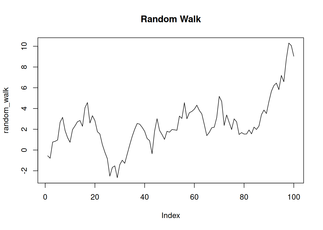
# Simulate seasonal data with noise
time <- 1:100
seasonal_data <- 10 * sin(2 * pi * time / 12) + rnorm(100, sd = 2)
plot(time, seasonal_data, type = "l", main = "Seasonal Data")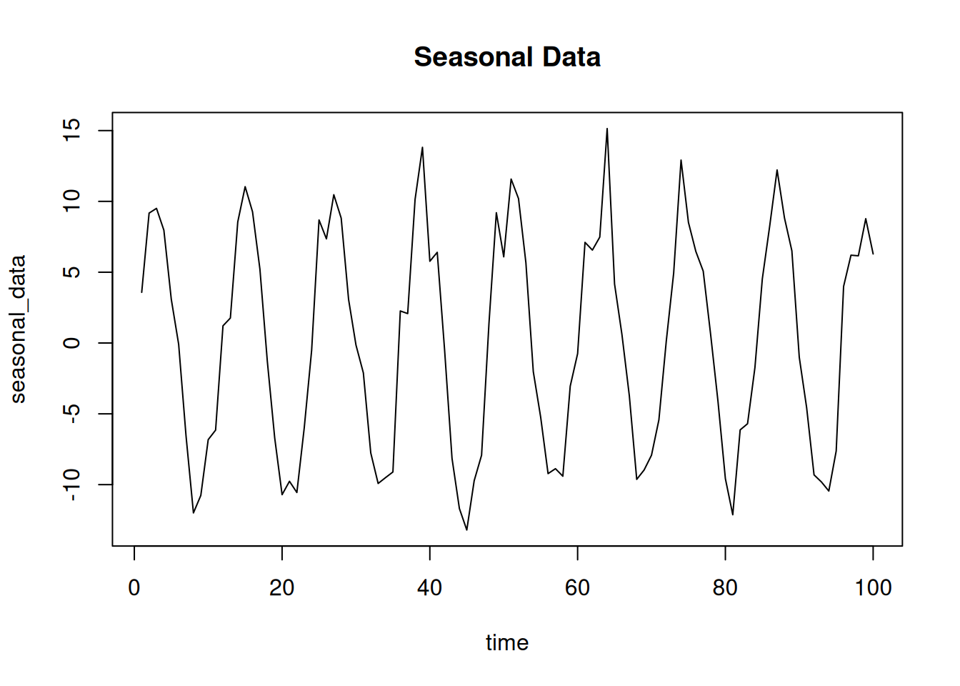
library(MASS)

# Define mean vector and covariance matrix
mu <- c(0, 0)
sigma <- matrix(c(1, 0.5, 0.5, 1), nrow = 2)

# Generate 100 samples
multivariate_data <- mvrnorm(n = 100, mu = mu, Sigma = sigma)
print(head(multivariate_data))
[,1] [,2]
[1,] 2.2618467 1.54660453
[2,] 1.5129275 0.76023849
[3,] 0.2396470 -0.69889171
[4,] 0.9966765 -0.05583679
[5,] -0.1402492 -0.57740869
[6,] -0.5780315 -0.24685232# Generate correlated data
set.seed(123)
x <- rnorm(100)
y <- 0.8 * x + rnorm(100, sd = 0.5)
plot(x, y, main = "Correlated Data")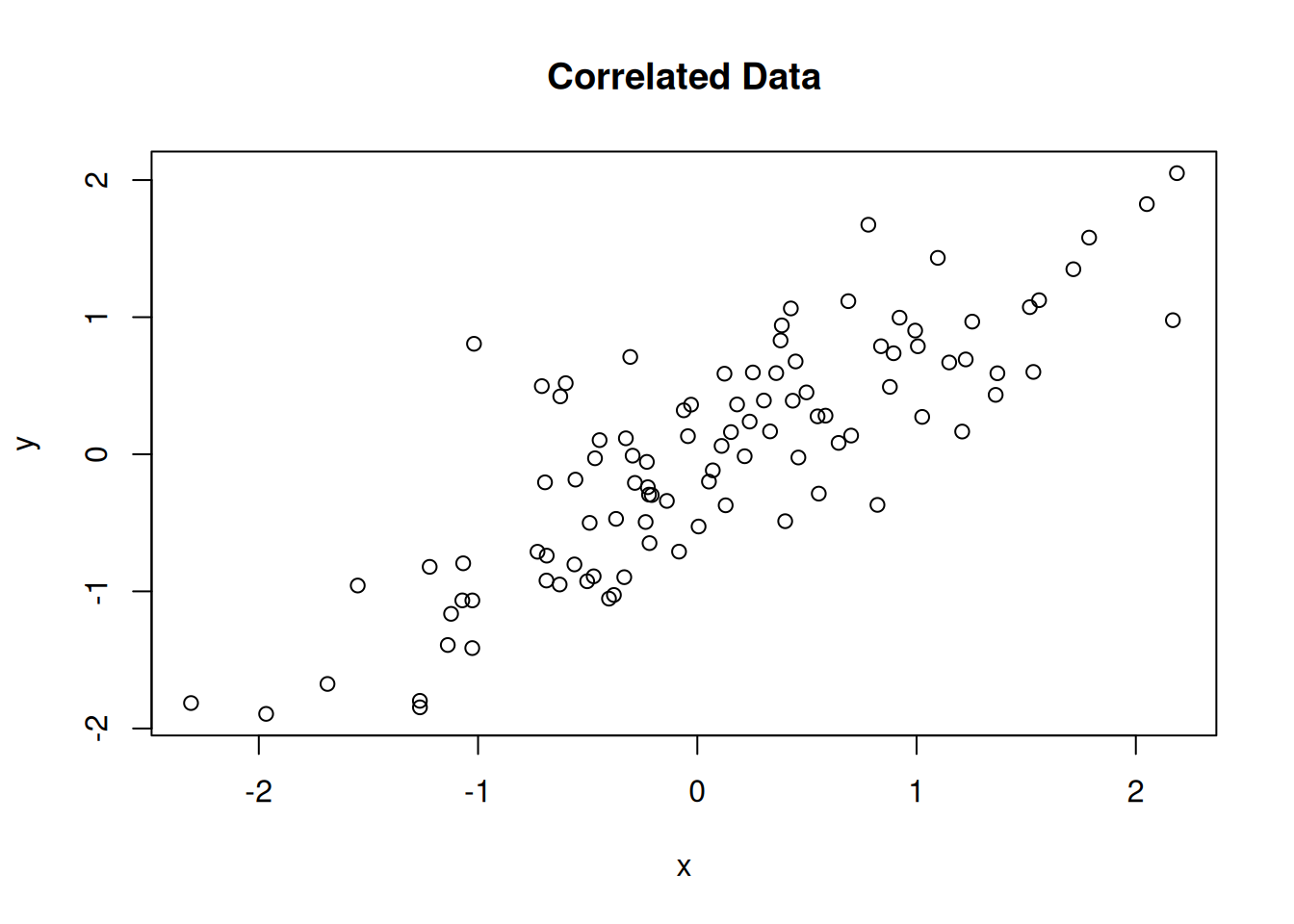
set.seed(123)

# Simulate a dataset with multiple types of variables
data <- data.frame(
  ID = 1:100,
  Age = sample(20:60, 100, replace = TRUE),
  Gender = sample(c("Male", "Female"), 100, replace = TRUE),
  Income = rnorm(100, mean = 50000, sd = 10000),
  Passed = sample(c(TRUE, FALSE), 100, replace = TRUE)
)
print(head(data))
ID Age Gender Income Passed
1 1 50 Male 52353.87 FALSE
2 2 34 Female 50779.61 FALSE
3 3 33 Male 40381.43 FALSE
4 4 22 Male 49286.92 TRUE
5 5 56 Male 64445.51 FALSE
6 6 33 Male 54515.04 FALSE# Add missing values to the Income column
data$Income[sample(1:100, 10)] <- NA
print(head(data)) ID Age Gender Income Passed
1 1 50 Male 52353.87 FALSE
2 2 34 Female 50779.61 FALSE
3 3 33 Male 40381.43 FALSE
4 4 22 Male 49286.92 TRUE
5 5 56 Male 64445.51 FALSE
6 6 33 Male NA FALSEMonte Carlo simulations involve repeated random sampling to compute a result.
set.seed(123)

# Simulate random points
n <- 10000
x <- runif(n, -1, 1)
y <- runif(n, -1, 1)

# Points inside the unit circle
inside_circle <- x^2 + y^2 <= 1
pi_estimate <- 4 * sum(inside_circle) / n
print(pi_estimate)
[1] 3.1576Bootstrapping involves resampling a dataset to estimate statistics.
set.seed(123)

# Original data
original_data <- rnorm(100, mean = 50, sd = 10)

# Bootstrap resamples
resamples <- replicate(1000, mean(sample(original_data, replace = TRUE)))
hist(resamples, main = "Bootstrap Means")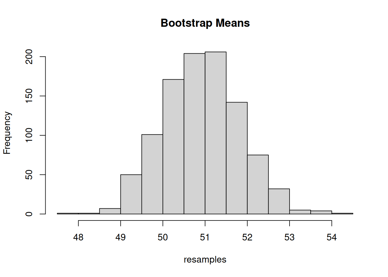
set.seed() to ensure reproducibility of random data.Simulating data in R is an essential skill that allows you to test ideas, compare methods, and better understand statistical principles. By mastering these techniques, you can create synthetic datasets tailored to your needs, whether for research, teaching, or debugging.