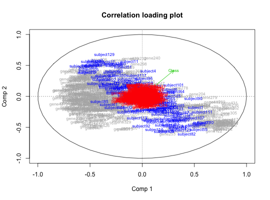
Correlation loadings plot for lpls regression model

This plot function produces a so-called correlation loadings plot. The correlation loadings are scaled versions of the regular loadings (and scores for X2) which make them informative in an overlayed plot. The plot enables better interpretation of the common covariance patterns in the three data matrices.

# S3 method for lplsReg
plot(x, comps = c(1, 2), doplot = c(TRUE, TRUE, TRUE),
  level = c(2, 2, 2), arrow = c(1, 0, 1), xlim = c(-1, 1), ylim = c(-1,
  1), samplecol = 4, pathcol = 2)

Arguments

x	A model x as returned from lplsReg
comps	a vector of length 2 indicating which components to be plotted, Default is the two first components.
doplot	A logical vector of length 3 indicating wether the correlation loadings for matrices X1, X2 and X3 should be plotted, respectively. Default is TRUe for all.
level	A numerical vector of length 3 where each element take the value 1 (plot symbol only) or 2 (plot variable labels) for matrix X1, X2 and X3, respectively.
arrow	A numerical vector of length 3 where each element take the value 0 (no arrow) or 1 (arrow from origin).
xlim	Limits for the x-axis
ylim	Limits for the y-axis
samplecol	The color used for the symbols for the "correlation scores" of X2.
pathcol	The color used for the correlation loading arrows (if arrow = 1) for X3.

Examples

data(BCdata)
fit <- lplsReg(BCdata$Y, BCdata$X, BCdata$Z, npc = 10)
plot(fit)